Slide 2

Mathematics is the science of the young. Otherwise it can not be. Mathematics is a form of mental gymnastics that requires all the flexibility and endurance of youth.

Norbert Wiener (1894-1964), American scientist

Slide 3

the relationship between the numbers a and b (mathematical expressions), connected by the signs Inequality -

Slide 4

Historical background Problems of proving equalities and inequalities arose in ancient times. Special words or their abbreviations were used to denote equality and inequality signs. IV century BC, Euclid, Book V of the Elements: if a, b, c, d are positive numbers and a is the largest number in the proportion a/b=c/d, then the inequality a+d=b holds +c. III century, the main work of Pappus of Alexandria “Mathematical collection”: if a, b, c, d are positive numbers and a/b>c/d, then the inequality ad>bc is satisfied.

More than 2000 BC the inequality was known turns into a true equality when a=b.

Slide 5

Modern special signs 1557. The equal sign = was introduced by the English mathematician R. Ricord. His motive: “No two objects can be more equal than two parallel segments.”

1631 Signs > and

Slide 6

Types of inequalities With a variable (one or more) Strict Non-strict With a modulus With a parameter Non-standard Systems Collections Numerical Simple Double Multiples Algebraic integers: -linear -quadratic -higher powers Fractional-rational Irrational Trigonometric Exponential Logarithmic Mixed type

is the value of a variable that, when substituted, turns it into a true numerical inequality. Solve an inequality - find all its solutions or prove that there are none. Two inequalities are said to be equivalent if all solutions to each are solutions to the other inequality or both inequalities have no solutions. Inequalities Solving inequalities in one variable

Slide 9

Describe the inequalities. Solve orally 3)(x – 2)(x + 3)  0

Slide 10

Graphical method

Solve graphically the inequality 1) Construct a graph 2) Construct a graph in the same coordinate system. 3) Find the abscissa of the intersection points of the graphs (the values ​​are taken approximately, we check the accuracy by substitution). 4) We determine from the graph the solution to this inequality. 5) Write down the answer.

Slide 11

Functional-graphical method for solving the inequality f(x)

Slide 12

Functional-graphical method Solve the inequality: 3) The equation f(x)=g(x) has at most one root. Solution. 4) By selection we find that x = 2. II. Let us schematically depict on the numerical axis Ox the graphs of the functions f (x) and g (x) passing through the point x = 2. III. Let's determine the solutions and write down the answer. Answer. x -7 undefined 2

Slide 13

Solve the inequalities:

Slide 14

Build graphs of the Unified State Examination-9 function, 2008

Slide 15

y x O 1 1 -1 -1 -2 -3 -4 2 3 4 -2 -3 -4 2 3 4 1) y=|x| 2) y=|x|-1 3) y=||x|-1| 4) y=||x|-1|-1 5) y=|||x|-1|-1| 6) y=|||x|-1|-1|-1 y=||||x|-1|-1|-1|

Slide 16

y x O 1 1 -1 -1 -2 -3 -4 2 3 4 -2 -3 -4 2 3 4 Determine the number of intervals of solutions to the inequality for each value of parameter a

Slide 17

Build a graph of the Unified State Examination-9 function, 2008

Slide 18

Slide 19

One of the most convenient methods for solving quadratic inequalities is the graphical method. In this article we will look at how quadratic inequalities are solved graphically. First, let's discuss what the essence of this method is. Next, we will present the algorithm and consider examples of solving quadratic inequalities graphically.

Page navigation.

The essence of the graphic method

At all graphical method for solving inequalities with one variable is used not only to solve quadratic inequalities, but also other types of inequalities. The essence graphic method solutions to inequalities next: consider the functions y=f(x) and y=g(x), which correspond to the left and right sides of the inequality, build their graphs in one rectangular coordinate system and find out at what intervals the graph of one of them is lower or higher than the other. Those intervals where

• the graph of the function f above the graph of the function g are solutions to the inequality f(x)>g(x) ;
• the graph of the function f not lower than the graph of the function g are solutions to the inequality f(x)≥g(x) ;
• the graph of f below the graph of g are solutions to the inequality f(x)
• the graph of a function f not higher than the graph of a function g are solutions to the inequality f(x)≤g(x) .

Let’s also say that the abscissas of the intersection points of the graphs of the functions f and g are solutions to the equation f(x)=g(x) .

Let's transfer these results to our case - to solve the quadratic inequality a x 2 +b x+c<0 (≤, >, ≥).

We introduce two functions: the first y=a x 2 +b x+c (with f(x)=a x 2 +b x+c) corresponding to the left side of the quadratic inequality, the second y=0 (with g (x)=0 ) corresponds to the right side of the inequality. Schedule quadratic function f is a parabola and the graph constant function g – straight line coinciding with the abscissa axis Ox.

Next, according to the graphical method of solving inequalities, it is necessary to analyze at what intervals the graph of one function is located above or below another, which will allow us to write down the desired solution to the quadratic inequality. In our case, we need to analyze the position of the parabola relative to the Ox axis.

Depending on the values ​​of the coefficients a, b and c, the following six options are possible (for our needs, a schematic representation is sufficient, and we do not need to depict the Oy axis, since its position does not affect the solutions to the inequality):

In this drawing we see a parabola, the branches of which are directed upward, and which intersects the Ox axis at two points, the abscissa of which are x 1 and x 2. This drawing corresponds to the option when the coefficient a is positive (it is responsible for the upward direction of the parabola branches), and when the value is positive discriminant of a quadratic trinomial a x 2 +b x+c (in this case, the trinomial has two roots, which we denoted as x 1 and x 2, and we assumed that x 1 0 , D=b 2 −4·a·c=(−1) 2 −4·1·(−6)=25>0, x 1 =−2 , x 2 =3 .

For clarity, let’s depict in red the parts of the parabola located above the x-axis, and in blue – those located below the x-axis.


Now let's find out which intervals correspond to these parts. The following drawing will help you identify them (in the future we will make similar selections in the form of rectangles mentally):


So on the abscissa axis two intervals (−∞, x 1) and (x 2 , +∞) were highlighted in red, on them the parabola is above the Ox axis, they constitute a solution to the quadratic inequality a x 2 +b x+c>0 , and the interval (x 1 , x 2) is highlighted in blue, there is a parabola below the Ox axis, it represents the solution to the inequality a x 2 +b x+c<0 . Решениями нестрогих квадратных неравенств a·x 2 +b·x+c≥0 и a·x 2 +b·x+c≤0 будут те же промежутки, но в них следует включить числа x 1 и x 2 , отвечающие равенству a·x 2 +b·x+c=0 .

And now briefly: for a>0 and D=b 2 −4 a c>0 (or D"=D/4>0 for an even coefficient b)

• the solution to the quadratic inequality a x 2 +b x+c>0 is (−∞, x 1)∪(x 2 , +∞) or in another notation x x 2 ;
• the solution to the quadratic inequality a x 2 +b x+c≥0 is (−∞, x 1 ]∪ or in another notation x 1 ≤x≤x 2 ,

where x 1 and x 2 are the roots of the square trinomial a x 2 +b x+c, and x 1


Here we see a parabola, the branches of which are directed upward, and which touches the abscissa axis, that is, it has one common point with it; we denote the abscissa of this point as x 0. The presented case corresponds to a>0 (the branches are directed upward) and D=0 (the square trinomial has one root x 0). For example, you can take the quadratic function y=x 2 −4·x+4, here a=1>0, D=(−4) 2 −4·1·4=0 and x 0 =2.

The drawing clearly shows that the parabola is located above the Ox axis everywhere except the point of contact, that is, on the intervals (−∞, x 0), (x 0, ∞). For clarity, let’s highlight areas in the drawing by analogy with the previous paragraph.


We draw conclusions: for a>0 and D=0

• the solution to the quadratic inequality a·x 2 +b·x+c>0 is (−∞, x 0)∪(x 0, +∞) or in another notation x≠x 0;
• the solution to the quadratic inequality a·x 2 +b·x+c≥0 is (−∞, +∞) or in another notation x∈R ;
• quadratic inequality a x 2 +b x+c<0 не имеет решений (нет интервалов, на которых парабола расположена ниже оси Ox );
• the quadratic inequality a x 2 +b x+c≤0 has a unique solution x=x 0 (it is given by the point of tangency),

where x 0 is the root of the square trinomial a x 2 + b x + c.


In this case, the branches of the parabola are directed upward, and it does not have common points with the abscissa axis. Here we have the conditions a>0 (branches are directed upward) and D<0 (квадратный трехчлен не имеет действительных корней). Для примера можно построить график функции y=2·x 2 +1 , здесь a=2>0 , D=0 2 −4·2·1=−8<0 .

Obviously, the parabola is located above the Ox axis throughout its entire length (there are no intervals at which it is below the Ox axis, there is no point of tangency).


Thus, for a>0 and D<0 решением квадратных неравенств a·x 2 +b·x+c>0 and a x 2 +b x+c≥0 is the set of all real numbers, and the inequalities a x 2 +b x+c<0 и a·x 2 +b·x+c≤0 не имеют решений.

And there remain three options for the location of the parabola with branches directed downward, not upward, relative to the Ox axis. In principle, they need not be considered, since multiplying both sides of the inequality by −1 allows us to go to an equivalent inequality with a positive coefficient for x 2. But it still doesn’t hurt to get an idea about these cases. The reasoning here is similar, so we will write down only the main results.

Solution algorithm

The result of all previous calculations is algorithm for solving quadratic inequalities graphically:

A schematic drawing is made on the coordinate plane, which depicts the Ox axis (it is not necessary to depict the Oy axis) and a sketch of a parabola corresponding to the quadratic function y=a·x 2 +b·x+c. To draw a sketch of a parabola, it is enough to find out two things:

• Firstly, by the value of the coefficient a it is determined where its branches are directed (for a>0 - upward, for a<0 – вниз).
• And secondly, by the value of the discriminant of the square trinomial a x 2 + b x + c it is determined whether the parabola intersects the abscissa axis at two points (for D>0), touches it at one point (for D=0), or has no common points with the Ox axis (at D<0 ). Для удобства на чертеже указываются координаты точек пересечения или координата точки касания (при наличии этих точек), а сами точки изображаются выколотыми при решении строгих неравенств, или обычными при решении нестрогих неравенств.

• When the drawing is ready, use it in the second step of the algorithm

  • when solving the quadratic inequality a·x 2 +b·x+c>0, the intervals are determined at which the parabola is located above the abscissa;
  • when solving the inequality a·x 2 +b·x+c≥0, the intervals at which the parabola is located above the abscissa axis are determined and the abscissas of the intersection points (or the abscissa of the tangent point) are added to them;
  • when solving the inequality a x 2 +b x+c<0 находятся промежутки, на которых парабола ниже оси Ox ;
  • finally, when solving a quadratic inequality of the form a·x 2 +b·x+c≤0, intervals are found in which the parabola is below the Ox axis and the abscissa of the intersection points (or the abscissa of the tangent point) is added to them;

  they constitute the desired solution to the quadratic inequality, and if there are no such intervals and no points of tangency, then the original quadratic inequality has no solutions.

All that remains is to solve a few quadratic inequalities using this algorithm.

Examples with solutions

Example.

Solve the inequality .

Solution.

We need to solve a quadratic inequality, let's use the algorithm from the previous paragraph. In the first step we need to draw a sketch of the graph of the quadratic function . The coefficient of x 2 is 2, it is positive, therefore, the branches of the parabola are directed upward. Let’s also find out whether the parabola has common points with the x-axis; to do this, we’ll calculate the discriminant of the quadratic trinomial . We have . The discriminant turned out to be greater than zero, therefore, the trinomial has two real roots: And , that is, x 1 =−3 and x 2 =1/3.

From this it is clear that the parabola intersects the Ox axis at two points with abscissas −3 and 1/3. We will depict these points in the drawing as ordinary points, since we are solving a non-strict inequality. Based on the clarified data, we obtain the following drawing (it fits the first template from the first paragraph of the article):

Let's move on to the second step of the algorithm. Since we are solving a non-strict quadratic inequality with the sign ≤, we need to determine the intervals at which the parabola is located below the abscissa axis and add to them the abscissas of the intersection points.

From the drawing it is clear that the parabola is below the x-axis on the interval (−3, 1/3) and to it we add the abscissas of the intersection points, that is, the numbers −3 and 1/3. As a result, we arrive at the numerical interval [−3, 1/3] . This is the solution we are looking for. It can be written as a double inequality −3≤x≤1/3.

Answer:

[−3, 1/3] or −3≤x≤1/3 .

Example.

Find the solution to the quadratic inequality −x 2 +16 x−63<0 .

Solution.

As usual, we start with a drawing. The numerical coefficient for the square of the variable is negative, −1, therefore, the branches of the parabola are directed downward. Let's calculate the discriminant, or better yet, its fourth part: D"=8 2 −(−1)·(−63)=64−63=1. Its value is positive, let's calculate the roots of the square trinomial: And , x 1 =7 and x 2 =9. So the parabola intersects the Ox axis at two points with abscissas 7 and 9 (the original inequality is strict, so we will depict these points with an empty center). Now we can make a schematic drawing:

Since we are solving a strict quadratic inequality with a sign<, то нас интересуют промежутки, на которых парабола расположена ниже оси абсцисс:

The drawing shows that the solutions to the original quadratic inequality are two intervals (−∞, 7) , (9, +∞) .

Answer:

(−∞, 7)∪(9, +∞) or in another notation x<7 , x>9 .

When solving quadratic inequalities, when the discriminant of a quadratic trinomial on its left side is zero, you need to be careful about including or excluding the abscissa of the tangent point from the answer. This depends on the sign of the inequality: if the inequality is strict, then it is not a solution to the inequality, but if it is not strict, then it is.

Example.

Does the quadratic inequality 10 x 2 −14 x+4.9≤0 have at least one solution?

Solution.

Let's plot the function y=10 x 2 −14 x+4.9. Its branches are directed upward, since the coefficient of x 2 is positive, and it touches the abscissa axis at the point with the abscissa 0.7, since D"=(−7) 2 −10 4.9=0, whence or 0.7 in the form of a decimal fraction. Schematically it looks like this:

Since we are solving a quadratic inequality with the ≤ sign, its solution will be the intervals on which the parabola is below the Ox axis, as well as the abscissa of the tangent point. From the drawing it is clear that there is not a single gap where the parabola would be below the Ox axis, so its solution will be only the abscissa of the tangent point, that is, 0.7.

Answer:

this inequality has a unique solution 0.7.

Example.

Solve the quadratic inequality –x 2 +8 x−16<0 .

Solution.

We follow the algorithm for solving quadratic inequalities and start by constructing a graph. The branches of the parabola are directed downward, since the coefficient of x 2 is negative, −1. Let us find the discriminant of the square trinomial –x 2 +8 x−16, we have D’=4 2 −(−1)·(−16)=16−16=0 and then x 0 =−4/(−1) , x 0 =4 . So, the parabola touches the Ox axis at the abscissa point 4. Let's make the drawing:

We look at the sign of the original inequality, it is there<. Согласно алгоритму, решение неравенства в этом случае составляют все промежутки, на которых парабола расположена строго ниже оси абсцисс.

In our case, these are open rays (−∞, 4) , (4, +∞) . Separately, we note that 4 - the abscissa of the point of contact - is not a solution, since at the point of contact the parabola is not lower than the Ox axis.

Answer:

(−∞, 4)∪(4, +∞) or in another notation x≠4 .

Pay special attention to cases where the discriminant of the quadratic trinomial on the left side of the quadratic inequality is less than zero. There is no need to rush here and say that the inequality has no solutions (we are used to making such a conclusion for quadratic equations with a negative discriminant). The point is that the quadratic inequality for D<0 может иметь решение, которым является множество всех действительных чисел.

Example.

Find the solution to the quadratic inequality 3 x 2 +1>0.

Solution.

As usual, we start with a drawing. The coefficient a is 3, it is positive, therefore, the branches of the parabola are directed upward. We calculate the discriminant: D=0 2 −4·3·1=−12 . Since the discriminant is negative, the parabola has no common points with the Ox axis. The information obtained is sufficient for a schematic graph:

We solve a strict quadratic inequality with a > sign. Its solution will be all intervals in which the parabola is above the Ox axis. In our case, the parabola is above the x-axis along its entire length, so the desired solution will be the set of all real numbers.

Ox , and also to them you need to add the abscissa of the points of intersection or the abscissa of the point of tangency. But the drawing clearly shows that there are no such gaps (since the parabola is everywhere below the abscissa axis), just as there are no points of intersection, and there are no points of tangency. Therefore, the original quadratic inequality has no solutions.

Answer:

no solutions or in another entry ∅.

Bibliography.

• Algebra: textbook for 8th grade. general education institutions / [Yu. N. Makarychev, N. G. Mindyuk, K. I. Neshkov, S. B. Suvorova]; ed. S. A. Telyakovsky. - 16th ed. - M.: Education, 2008. - 271 p. : ill. - ISBN 978-5-09-019243-9.
• Algebra: 9th grade: educational. for general education institutions / [Yu. N. Makarychev, N. G. Mindyuk, K. I. Neshkov, S. B. Suvorova]; ed. S. A. Telyakovsky. - 16th ed. - M.: Education, 2009. - 271 p. : ill. - ISBN 978-5-09-021134-5.
• Mordkovich A. G. Algebra. 8th grade. In 2 hours. Part 1. Textbook for students of general education institutions / A. G. Mordkovich. - 11th ed., erased. - M.: Mnemosyne, 2009. - 215 p.: ill. ISBN 978-5-346-01155-2.
• Mordkovich A. G. Algebra. 9th grade. In 2 hours. Part 1. Textbook for students of general education institutions / A. G. Mordkovich, P. V. Semenov. - 13th ed., erased. - M.: Mnemosyne, 2011. - 222 p.: ill. ISBN 978-5-346-01752-3.
• Mordkovich A. G. Algebra and beginning of mathematical analysis. Grade 11. In 2 parts. Part 1. Textbook for students of general education institutions (profile level) / A. G. Mordkovich, P. V. Semenov. - 2nd ed., erased. - M.: Mnemosyne, 2008. - 287 p.: ill. ISBN 978-5-346-01027-2.

Graphical solution of equations

Heyday, 2009

Introduction

The need to solve quadratic equations in ancient times was caused by the need to solve problems related to finding the areas of land and with military excavation work, as well as with the development of astronomy and mathematics itself. The Babylonians were able to solve quadratic equations around 2000 BC. The rule for solving these equations, set out in the Babylonian texts, essentially coincides with modern ones, but it is not known how the Babylonians arrived at this rule.

Formulas for solving quadratic equations in Europe were first set forth in the Book of Abacus, written in 1202 by the Italian mathematician Leonardo Fibonacci. His book contributed to the spread of algebraic knowledge not only in Italy, but also in Germany, France and other European countries.

But the general rule for solving quadratic equations, with all possible combinations of coefficients b and c, was formulated in Europe only in 1544 by M. Stiefel.

In 1591 Francois Viet introduced formulas for solving quadratic equations.

In ancient Babylon they could solve some types of quadratic equations.

Diophantus of Alexandria And Euclid, Al-Khwarizmi And Omar Khayyam solved equations using geometric and graphical methods.

In 7th grade we studied functions y = C, y =kx, y =kx+ m, y =x 2,y = –x 2, in 8th grade - y = √x, y =|x|, y =ax2 + bx+ c, y =k/ x. In the 9th grade algebra textbook, I saw functions that were not yet known to me: y =x 3, y =x 4,y =x 2n, y =x- 2n, y = 3√x, (x– a) 2 + (y –b) 2 = r 2 and others. There are rules for constructing graphs of these functions. I wondered if there were other functions that obey these rules.

My job is to study function graphs and solve equations graphically.

1. What are the functions?

The graph of a function is the set of all points of the coordinate plane, the abscissas of which are equal to the values ​​of the arguments, and the ordinates are equal to the corresponding values ​​of the function.

The linear function is given by the equation y =kx+ b, Where k And b- some numbers. The graph of this function is a straight line.

Inverse proportional function y =k/ x, where k ¹ 0. The graph of this function is called a hyperbola.

Function (x– a) 2 + (y –b) 2 = r2 , Where A, b And r- some numbers. The graph of this function is a circle of radius r with center at point A ( A, b).

Quadratic function y= ax2 + bx+ c Where A,b, With– some numbers and A¹ 0. The graph of this function is a parabola.

The equation at2 (a– x) = x2 (a+ x) . The graph of this equation will be a curve called a strophoid.

/>Equation (x2 + y2 ) 2 = a(x2 – y2 ) . The graph of this equation is called Bernoulli's lemniscate.

The equation. The graph of this equation is called an astroid.

Curve (x2 y2 – 2 ax)2 =4 a2 (x2 + y2 ) . This curve is called a cardioid.

Functions: y =x 3 – cubic parabola, y =x 4, y = 1/x 2.

2. The concept of an equation and its graphical solution

The equation– an expression containing a variable.

Solve the equation- this means finding all its roots, or proving that they do not exist.

Root of the equation is a number that, when substituted into an equation, produces a correct numerical equality.

Solving equations graphically allows you to find the exact or approximate value of the roots, allows you to find the number of roots of the equation.

When constructing graphs and solving equations, the properties of a function are used, which is why the method is often called functional-graphical.

To solve, we “divide” the equation into two parts, introduce two functions, construct their graphs, and find the coordinates of the points of intersection of the graphs. The abscissas of these points are the roots of the equation.

3. Algorithm for constructing a graph of a function

Knowing the graph of a function y =f(x) , you can build graphs of functions y =f(x+ m) ,y =f(x)+ l And y =f(x+ m)+ l. All these graphs are obtained from the graph of the function y =f(x) using parallel carry transformation: to │ m│ units of scale to the right or left along the x-axis and on │ l│ units of scale up or down along an axis y.

4. Graphical solution of the quadratic equation

Using a quadratic function as an example, we will consider the graphical solution of a quadratic equation. The graph of a quadratic function is a parabola.

What did the ancient Greeks know about the parabola?

Modern mathematical symbolism originated in the 16th century.

The ancient Greek mathematicians had neither the coordinate method nor the concept of function. Nevertheless, the properties of the parabola were studied in detail by them. The ingenuity of ancient mathematicians is simply amazing - after all, they could only use drawings and verbal descriptions of dependencies.

Most fully explored the parabola, hyperbola and ellipse Apollonius of Perga, who lived in the 3rd century BC. He gave these curves names and indicated what conditions the points lying on this or that curve satisfy (after all, there were no formulas!).

There is an algorithm for constructing a parabola:

Find the coordinates of the vertex of the parabola A (x0; y0): X=- b/2 a;

y0=axo2+in0+s;

Find the axis of symmetry of the parabola (straight line x=x0);

PAGE_BREAK--

We compile a table of values ​​for constructing control points;

We construct the resulting points and construct points that are symmetrical to them relative to the axis of symmetry.

1. Using the algorithm, we will construct a parabola y= x2 – 2 x– 3 . Abscissas of points of intersection with the axis x and there are roots of the quadratic equation x2 – 2 x– 3 = 0.

There are five ways to solve this equation graphically.

2. Let's split the equation into two functions: y= x2 And y= 2 x+ 3

3. Let's split the equation into two functions: y= x2 –3 And y=2 x. The roots of the equation are the abscissas of the points of intersection of the parabola and the line.

4. Transform the equation x2 – 2 x– 3 = 0 by isolating a complete square into functions: y= (x–1) 2 And y=4. The roots of the equation are the abscissas of the points of intersection of the parabola and the line.

5. Divide both sides of the equation term by term x2 – 2 x– 3 = 0 on x, we get x– 2 – 3/ x= 0 , let's split this equation into two functions: y= x– 2, y= 3/ x. The roots of the equation are the abscissas of the points of intersection of the line and the hyperbola.

5. Graphical solution of degree equationsn

Example 1. Solve the equation x5 = 3 – 2 x.

y= x5 , y= 3 – 2 x.

Answer: x = 1.

Example 2. Solve the equation 3 √ x= 10 – x.

The roots of this equation are the abscissa of the point of intersection of the graphs of two functions: y= 3 √ x, y= 10 – x.

Answer: x = 8.

Conclusion

Having looked at the graphs of the functions: y =ax2 + bx+ c, y =k/ x, у = √x, y =|x|, y =x 3, y =x 4,y = 3√x, I noticed that all these graphs are built according to the rule of parallel translation relative to the axes x And y.

Using the example of solving a quadratic equation, we can conclude that the graphical method is also applicable for equations of degree n.

Graphical methods for solving equations are beautiful and understandable, but do not provide a 100% guarantee of solving any equation. The abscissas of the intersection points of the graphs can be approximate.

In 9th grade and throughout high school, I will continue to explore other functions. I'm interested to know whether those functions obey the rules of parallel transfer when plotting their graphs.

Next year I would also like to consider the issues of graphically solving systems of equations and inequalities.

Literature

1. Algebra. 7th grade. Part 1. Textbook for educational institutions / A.G. Mordkovich. M.: Mnemosyne, 2007.

2. Algebra. 8th grade. Part 1. Textbook for educational institutions / A.G. Mordkovich. M.: Mnemosyne, 2007.

3. Algebra. 9th grade. Part 1. Textbook for educational institutions / A.G. Mordkovich. M.: Mnemosyne, 2007.

4. Glazer G.I. History of mathematics at school. VII–VIII grades. – M.: Education, 1982.

5. Journal Mathematics No. 5 2009; No. 8 2007; No. 23 2008.

6. Graphical solution of equations websites on the Internet: Tol VIKI; stimul.biz/ru; wiki.iot.ru/images; berdsk.edu; page 3–6.htm.

Ministry of Education and Youth Policy of the Stavropol Territory

State budgetary professional educational institution

Georgievsk Regional College "Integral"

INDIVIDUAL PROJECT

In the discipline “Mathematics: algebra, principles of mathematical analysis, geometry”

On the topic: “Graphical solution of equations and inequalities”

Completed by a student of group PK-61, studying in the specialty

"Programming in computer systems"

Zeller Timur Vitalievich

Head: teacher Serkova N.A.

Submission date:" " 2017

Defense date:" " 2017

Georgievsk 2017

EXPLANATORY NOTE

OBJECTIVE OF THE PROJECT:

Target: Find out the advantages of the graphical method of solving equations and inequalities.

Tasks:

Compare the analytical and graphical methods of solving equations and inequalities.

Find out in what cases the graphical method has advantages.

Consider solving equations with modulus and parameter.

The relevance of research: Analysis of the material devoted to the graphic solution of equations and inequalities in the textbooks “Algebra and the beginnings of mathematical analysis” by various authors, taking into account the goals of studying this topic. As well as mandatory learning outcomes related to the topic under consideration.

Content

Introduction

1. Equations with parameters

1.1. Definitions

1.2. Solution algorithm

1.3. Examples

2. Inequalities with parameters

2.1. Definitions

2.2. Solution algorithm

2.3. Examples

3. Using graphs in solving equations

3.1. Graphical solution of a quadratic equation

3.2. Systems of equations

3.3. Trigonometric equations

4. Application of graphs in solving inequalities

5.Conclusion

6. References

Introduction

The study of many physical processes and geometric patterns often leads to solving problems with parameters. Some universities also include equations, inequalities and their systems in exam papers, which are often very complex and require a non-standard approach to solution. At school, this one of the most difficult sections of the school mathematics course is considered only in a few elective classes.

In preparing this work, I set the goal of a deeper study of this topic, identifying the most rational solution that quickly leads to an answer. In my opinion, the graphical method is a convenient and fast way to solve equations and inequalities with parameters.

My project examines frequently encountered types of equations, inequalities and their systems.

1. Equations with parameters

1. Basic definitions

Consider the equation

(a, b, c, …, k, x)=(a, b, c, …, k, x), (1)

where a, b, c, …, k, x are variable quantities.

Any system of variable values

a = a 0 , b = b 0 , c = c 0 , …, k = k 0 , x = x 0 ,

in which both the left and right sides of this equation take real values ​​is called a system of permissible values ​​of the variables a, b, c, ..., k, x. Let A be the set of all admissible values ​​of a, B be the set of all admissible values ​​of b, etc., X be the set of all admissible values ​​of x, i.e. aA, bB, …, xX. If for each of the sets A, B, C, …, K we select and fix, respectively, one value a, b, c, …, k and substitute them into equation (1), then we obtain an equation for x, i.e. equation with one unknown.

The variables a, b, c, ..., k, which are considered constant when solving an equation, are called parameters, and the equation itself is called an equation containing parameters.

The parameters are designated by the first letters of the Latin alphabet: a, b, c, d, ..., k, l, m, n, and the unknowns are designated by the letters x, y, z.

To solve an equation with parameters means to indicate at what values ​​of the parameters solutions exist and what they are.

Two equations containing the same parameters are called equivalent if:

a) they make sense for the same parameter values;

b) every solution to the first equation is a solution to the second and vice versa.

1. Solution algorithm

Find the domain of definition of the equation.

We express a as a function of x.

In the xOa coordinate system, we construct a graph of the function a=(x) for those values ​​of x that are included in the domain of definition of this equation.

We find the intersection points of the straight line a=c, where c(-;+) with the graph of the function a=(x). If the straight line a=c intersects the graph a=(x), then we determine the abscissas of the intersection points. To do this, it is enough to solve the equation a=(x) for x.

We write down the answer.

1. Examples

I. Solve the equation

(1)

Solution.

Since x=0 is not a root of the equation, the equation can be resolved for a:

or

The graph of a function is two “glued” hyperbolas. The number of solutions to the original equation is determined by the number of intersection points of the constructed line and the straight line y=a.

If a  (-;-1](1;+) , then the straight line y=a intersects the graph of equation (1) at one point. We will find the abscissa of this point when solving the equation for x.

Thus, on this interval, equation (1) has a solution.

If a , then the straight line y=a intersects the graph of equation (1) at two points. The abscissas of these points can be found from the equations and, we get

And.

If a , then the straight line y=a does not intersect the graph of equation (1), therefore there are no solutions.

Answer:

If a  (-;-1](1;+), then;

If a  , then ;

If a  , then there are no solutions.

II. Find all values ​​of the parameter a for which the equation has three different roots.

Solution.

Having rewritten the equation in the form and considered a pair of functions, you can notice that the desired values ​​of the parameter a and only they will correspond to those positions of the function graph at which it has exactly three points of intersection with the function graph.

In the xOy coordinate system, we will construct a graph of the function). To do this, we can represent it in the form and, having considered four arising cases, we write this function in the form

Since the graph of a function is a straight line that has an angle of inclination to the Ox axis equal to and intersects the Oy axis at a point with coordinates (0, a), we conclude that the three indicated intersection points can be obtained only in the case when this line touches the graph of the function. Therefore we find the derivative

Answer: .

III. Find all values ​​of the parameter a, for each of which the system of equations

has solutions.

Solution.

From the first equation of the system we obtain at Therefore, this equation defines a family of “semi-parabolas” - the right branches of the parabola “slide” with their vertices along the abscissa axis.

Let's select complete squares on the left side of the second equation and factorize it

The set of points of the plane satisfying the second equation are two straight lines

Let us find out at what values ​​of the parameter a a curve from the family of “semiparabolas” has at least one common point with one of the resulting straight lines.

If the vertices of the semiparabolas are to the right of point A, but to the left of point B (point B corresponds to the vertex of the “semiparabola” that touches

straight line), then the graphs under consideration do not have common points. If the vertex of the “semiparabola” coincides with point A, then.

We determine the case of a “semiparabola” touching a line from the condition of the existence of a unique solution to the system

In this case, the equation

has one root, from where we find:

Consequently, the original system has no solutions at, but at or has at least one solution.

Answer: a  (-;-3] (;+).

IV. Solve the equation

Solution.

Using equality, we rewrite the given equation in the form

This equation is equivalent to the system

We rewrite the equation in the form

. (*)

The last equation is easiest to solve using geometric considerations. Let's construct graphs of the functions and From the graph it follows that the graphs do not intersect and, therefore, the equation has no solutions.

If, then when the graphs of the functions coincide and, therefore, all values ​​are solutions to equation (*).

When the graphs intersect at one point, the abscissa of which is. Thus, when equation (*) has a unique solution - .

Let us now investigate at what values ​​of a the found solutions to equation (*) will satisfy the conditions

Let it be then. The system will take the form

Its solution will be the interval x (1;5). Considering that, we can conclude that if the original equation is satisfied by all values ​​of x from the interval, the original inequality is equivalent to the correct numerical inequality 2<4.Поэтому все значения переменной, принадлежащие этому отрезку, входят в множество решений.

On the integral (1;+∞) we again obtain the linear inequality 2х<4, справедливое при х<2. Поэтому интеграл (1;2) также входит в множество решений. Объединяя полученные результаты, делаем вывод: неравенству удовлетворяют все значения переменной из интеграла (-2;2) и только они.

However, the same result can be obtained from visual and at the same time strict geometric considerations. Figure 7 shows the function graphs:y= f( x)=| x-1|+| x+1| Andy=4.

Figure 7.

On the integral (-2;2) graph of the functiony= f(x) is located under the graph of the function y=4, which means that the inequalityf(x)<4 справедливо. Ответ:(-2;2)

II )Inequalities with parameters.

Solving inequalities with one or more parameters is, as a rule, a more complex task compared to a problem in which there are no parameters.

For example, the inequality √a+x+√a-x>4, which contains the parameter a, naturally requires much more effort to solve than the inequality √1+x + √1-x>1.

What does it mean to solve the first of these inequalities? This, in essence, means solving not just one inequality, but a whole class, a whole set of inequalities that are obtained if we give the parameter a specific numerical values. The second of the written inequalities is a special case of the first, since it is obtained from it with the value a = 1.

Thus, to solve an inequality containing parameters means to determine at what values ​​of the parameters the inequality has solutions and for all such parameter values ​​to find all the solutions.

Example1:

Solve the inequality |x-a|+|x+a|< b, a<>0.

To solve this inequality with two parametersa u bLet's use geometric considerations. Figures 8 and 9 show the function graphs.

Y= f(x)=| x- a|+| x+ a| u y= b.

It is obvious that whenb<=2| a| straighty= bdoes not pass above the horizontal segment of the curvey=| x- a|+| x+ a| and, therefore, the inequality in this case has no solutions (Figure 8). Ifb>2| a|, then the liney= bintersects the graph of a functiony= f(x) at two points (-b/2; b) u (b/2; b)(Figure 6) and the inequality in this case is valid for –b/2< x< b/2, since for these values ​​of the variable the curvey=| x+ a|+| x- a| located under the straight liney= b.

Answer: Ifb<=2| a| , then there are no solutions,

Ifb>2| a|, thenx €(- b/2; b/2).

III) Trigonometric inequalities:

When solving inequalities with trigonometric functions, the periodicity of these functions and their monotonicity on the corresponding intervals are essentially used. The simplest trigonometric inequalities. Functionsin xhas a positive period of 2π. Therefore, inequalities of the form:sin x>a, sin x>=a,

sin x

It is enough to solve first on some segment of length 2π . We obtain the set of all solutions by adding to each of the solutions found on this segment numbers of the form 2π p, pЄZ.

Example 1: Solve inequalitysin x>-1/2.(Figure 10)

First, let's solve this inequality on the interval [-π/2;3π/2]. Let's consider its left side - the segment [-π/2;3π/2]. Here is the equationsin x=-1/2 has one solution x=-π/6; and the functionsin xincreases monotonically. This means that if –π/2<= x<= -π/6, то sin x<= sin(- π /6)=-1/2, i.e. these values ​​of x are not solutions to the inequality. If –π/6<х<=π/2 то sin x> sin(-π/6) = –1/2. All these values ​​of x are not solutions to the inequality.

On the remaining segment [π/2;3π/2] the functionsin xthe equation also decreases monotonicallysin x= -1/2 has one solution x=7π/6. Therefore, if π/2<= x<7π/, то sin x> sin(7π/6)=-1/2, i.e. all these values ​​of x are solutions to the inequality. ForxWe havesin x<= sin(7π/6)=-1/2, these x values ​​are not solutions. Thus, the set of all solutions to this inequality on the interval [-π/2;3π/2] is the integral (-π/6;7π/6).

Due to the periodicity of the functionsin xwith a period of 2π values ​​of x from any integral of the form: (-π/6+2πn;7π/6 +2πn),nЄZ, are also solutions to the inequality. No other values ​​of x are solutions to this inequality.

Answer: -π/6+2πn< x<7π/6+2π n, WherenЄ Z.

Conclusion

We looked at the graphical method for solving equations and inequalities; We looked at specific examples, the solution of which used such properties of functions as monotonicity and parity.Analysis of scientific literature and mathematics textbooks made it possible to structure the selected material in accordance with the objectives of the study, select and develop effective methods for solving equations and inequalities. The paper presents a graphical method for solving equations and inequalities and examples in which these methods are used. The result of the project can be considered creative tasks, as auxiliary material for developing the skill of solving equations and inequalities using the graphical method.

List of used literature

Dalinger V. A. “Geometry helps algebra.” Publishing house “School - Press”. Moscow 1996

Dalinger V. A. “Everything to ensure success in final and entrance exams in mathematics.” Publishing house of Omsk Pedagogical University. Omsk 1995

Okunev A. A. “Graphical solution of equations with parameters.” Publishing house “School - Press”. Moscow 1986

Pismensky D. T. “Mathematics for high school students.” Publishing house “Iris”. Moscow 1996

Yastribinetsky G. A. “Equations and inequalities containing parameters.” Publishing house “Prosveshcheniye”. Moscow 1972

G. Korn and T. Korn “Handbook of Mathematics.” Publishing house “Science” physical and mathematical literature. Moscow 1977

Amelkin V.V. and Rabtsevich V.L. “Problems with parameters”. Publishing house “Asar”. Minsk 1996

Internet resources

The graphical method is one of the main methods for solving quadratic inequalities. In the article we will present an algorithm for using the graphical method, and then consider special cases using examples.

The essence of the graphical method

The method is applicable to solving any inequalities, not only quadratic ones. Its essence is this: the right and left sides of the inequality are considered as two separate functions y = f (x) and y = g (x), their graphs are plotted in a rectangular coordinate system and look at which of the graphs is located above the other, and on which intervals. The intervals are assessed as follows:

Definition 1

• solutions to the inequality f (x) > g (x) are intervals where the graph of the function f is higher than the graph of the function g;
• solutions to the inequality f (x) ≥ g (x) are intervals where the graph of the function f is not lower than the graph of the function g;
• solutions to the inequality f(x)< g (x) являются интервалы, где график функции f ниже графика функции g ;
• solutions to the inequality f (x) ≤ g (x) are intervals where the graph of the function f is not higher than the graph of the function g;
• The abscissas of the intersection points of the graphs of the functions f and g are solutions to the equation f (x) = g (x).

Let's look at the above algorithm using an example. To do this, take the quadratic inequality a x 2 + b x + c< 0 (≤ , >, ≥) and derive two functions from it. The left side of the inequality will correspond to y = a · x 2 + b · x + c (in this case f (x) = a · x 2 + b · x + c), and the right side y = 0 (in this case g (x) = 0).

The graph of the first function is a parabola, the second is a straight line, which coincides with the x-axis O x. Let's analyze the position of the parabola relative to the O x axis. To do this, let's make a schematic drawing.

The branches of the parabola are directed upward. It intersects the O x axis at points x 1 And x 2. Coefficient a in this case is positive, since it is it that is responsible for the direction of the branches of the parabola. The discriminant is positive, indicating that the quadratic trinomial has two roots a x 2 + b x + c. We denote the roots of the trinomial as x 1 And x 2, and it was accepted that x 1< x 2 , since a point with an abscissa is depicted on the O x axis x 1 to the left of the abscissa point x 2.

The parts of the parabola located above the O x axis will be denoted in red, below - in blue. This will allow us to make the drawing more visual.

Let's select the spaces that correspond to these parts and mark them in the picture with fields of a certain color.

We marked in red the intervals (− ∞, x 1) and (x 2, + ∞), on them the parabola is above the O x axis. They are a · x 2 + b · x + c > 0. We marked in blue the interval (x 1 , x 2), which is the solution to the inequality a x 2 + b x + c< 0 . Числа x 1 и x 2 будут отвечать равенству a · x 2 + b · x + c = 0 .

Let's make a brief summary of the solution. For a > 0 and D = b 2 − 4 a c > 0 (or D " = D 4 > 0 for an even coefficient b) we get:

• the solution to the quadratic inequality a x 2 + b x + c > 0 is (− ∞ , x 1) ∪ (x 2 , + ∞) or in another notation x< x 1 , x >x 2 ;
• the solution to the quadratic inequality a · x 2 + b · x + c ≥ 0 is (− ∞ , x 1 ] ∪ [ x 2 , + ∞) or in another form x ≤ x 1 , x ≥ x 2 ;
• solving the quadratic inequality a x 2 + b x + c< 0 является (x 1 , x 2) или в другой записи x 1 < x < x 2 ;
• the solution to the quadratic inequality a x 2 + b x + c ≤ 0 is [ x 1 , x 2 ] or in another notation x 1 ≤ x ≤ x 2 ,

where x 1 and x 2 are the roots of the quadratic trinomial a · x 2 + b · x + c, and x 1< x 2 .

In this figure, the parabola touches the O x axis only at one point, which is designated as x 0 a > 0. D=0, therefore, the quadratic trinomial has one root x 0.

The parabola is located above the O x axis completely, with the exception of the point of tangency of the coordinate axis. Let's color the intervals (− ∞ , x 0) , (x 0 , ∞) .

Let's write down the results. At a > 0 And D=0:

• solving the quadratic inequality a x 2 + b x + c > 0 is (− ∞ , x 0) ∪ (x 0 , + ∞) or in another notation x ≠ x 0;
• solving the quadratic inequality a x 2 + b x + c ≥ 0 is (− ∞ , + ∞) or in another notation x ∈ R;
• quadratic inequality a x 2 + b x + c< 0 has no solutions (there are no intervals at which the parabola is located below the axis O x);
• quadratic inequality a x 2 + b x + c ≤ 0 has a unique solution x = x 0(it is given by the point of contact),

Where x 0- root of the square trinomial a x 2 + b x + c.

Let's consider the third case, when the branches of the parabola are directed upward and do not touch the axis O x. The branches of the parabola are directed upward, which means that a > 0. The square trinomial has no real roots because D< 0 .

There are no intervals on the graph at which the parabola would be below the x-axis. We will take this into account when choosing a color for our drawing.

It turns out that when a > 0 And D< 0 solving quadratic inequalities a x 2 + b x + c > 0 And a x 2 + b x + c ≥ 0 is the set of all real numbers, and the inequalities a x 2 + b x + c< 0 And a x 2 + b x + c ≤ 0 have no solutions.

We have three options left to consider when the branches of the parabola are directed downward. There is no need to dwell on these three options in detail, since when we multiply both sides of the inequality by − 1, we obtain an equivalent inequality with a positive coefficient for x 2.

Consideration of the previous section of the article prepared us for the perception of an algorithm for solving inequalities using a graphical method. To carry out calculations, we will need to use a drawing each time, which will depict the coordinate line O x and a parabola that corresponds to the quadratic function y = a x 2 + b x + c. In most cases, we will not depict the O y axis, since it is not needed for calculations and will only overload the drawing.

To construct a parabola, we will need to know two things:

Definition 2

• the direction of the branches, which is determined by the value of the coefficient a;
• the presence of points of intersection of the parabola and the abscissa axis, which are determined by the value of the discriminant of the quadratic trinomial a · x 2 + b · x + c .

We will denote the points of intersection and tangency in the usual way when solving non-strict inequalities and empty when solving strict ones.

Having a completed drawing allows you to move on to the next step of the solution. It involves determining the intervals at which the parabola is located above or below the O x axis. The intervals and points of intersection are the solution to the quadratic inequality. If there are no points of intersection or tangency and there are no intervals, then it is considered that the inequality specified in the conditions of the problem has no solutions.

Now let's solve several quadratic inequalities using the above algorithm.

Example 1

It is necessary to solve the inequality 2 x 2 + 5 1 3 x - 2 graphically.

Solution

Let's draw a graph of the quadratic function y = 2 · x 2 + 5 1 3 · x - 2 . Coefficient at x 2 positive because it is equal 2 . This means that the branches of the parabola will be directed upward.

Let us calculate the discriminant of the quadratic trinomial 2 x 2 + 5 1 3 x - 2 in order to find out whether the parabola has common points with the abscissa axis. We get:

D = 5 1 3 2 - 4 2 (- 2) = 400 9

As we see, D is greater than zero, therefore, we have two intersection points: x 1 = - 5 1 3 - 400 9 2 2 and x 2 = - 5 1 3 + 400 9 2 2, that is, x 1 = − 3 And x 2 = 1 3.

We solve a non-strict inequality, therefore we put ordinary points on the graph. Let's draw a parabola. As you can see, the drawing has the same appearance as in the first template we considered.

Our inequality has the sign ≤. Therefore, we need to highlight the intervals on the graph in which the parabola is located below the O x axis and add intersection points to them.

The interval we need is 3, 1 3. We add intersection points to it and get a numerical segment − 3, 1 3. This is the solution to our problem. The answer can be written as a double inequality: − 3 ≤ x ≤ 1 3 .

Answer:− 3 , 1 3 or − 3 ≤ x ≤ 1 3 .

Example 2

− x 2 + 16 x − 63< 0 graphical method.

Solution

The square of the variable has a negative numerical coefficient, so the branches of the parabola will be directed downward. Let's calculate the fourth part of the discriminant D " = 8 2 − (− 1) · (− 63) = 64 − 63 = 1. This result tells us that there will be two points of intersection.

Let's calculate the roots of the quadratic trinomial: x 1 = - 8 + 1 - 1 and x 2 = - 8 - 1 - 1, x 1 = 7 and x 2 = 9.

It turns out that the parabola intersects the x-axis at the points 7 And 9 . Let's mark these points on the graph as empty, since we are working with strict inequality. After this, draw a parabola that intersects the O x axis at the marked points.

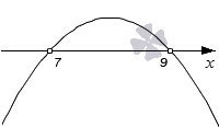
We will be interested in the intervals at which the parabola is located below the O x axis. Let's mark these intervals in blue.

We get the answer: the solution to the inequality is the intervals (− ∞ , 7) , (9 , + ∞) .

Answer:(− ∞ , 7) ∪ (9 , + ∞) or in another notation x< 7 , x > 9 .

In cases where the discriminant of a quadratic trinomial is zero, it is necessary to carefully consider whether to include the abscissa of the tangent points in the answer. In order to make the right decision, it is necessary to take into account the inequality sign. In strict inequalities, the point of tangency of the x-axis is not a solution to the inequality, but in non-strict ones it is.

Example 3

Solve quadratic inequality 10 x 2 − 14 x + 4, 9 ≤ 0 graphical method.

Solution

The branches of the parabola in this case will be directed upward. It will touch the O x axis at point 0, 7, since

Let's plot the function y = 10 x 2 − 14 x + 4.9. Its branches are directed upward, since the coefficient at x 2 positive, and it touches the x-axis at the x-axis point 0 , 7 , because D " = (− 7) 2 − 10 4, 9 = 0, from where x 0 = 7 10 or 0 , 7 .

Let's put a point and draw a parabola.

We solve a non-strict inequality with a sign ≤. Hence. We will be interested in the intervals at which the parabola is located below the x-axis and the point of tangency. There are no intervals in the figure that would satisfy our conditions. There is only a point of contact 0, 7. This is the solution we are looking for.

Answer: The inequality has only one solution 0, 7.

Example 4

Solve quadratic inequality – x 2 + 8 x − 16< 0 .

Solution

The branches of the parabola are directed downwards. The discriminant is zero. Intersection point x 0 = 4.

We mark the point of tangency on the x-axis and draw a parabola.

We are dealing with severe inequality. Consequently, we are interested in the intervals at which the parabola is located below the O x axis. Let's mark them in blue.

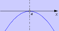
The point with abscissa 4 is not a solution, since the parabola at it is not located below the O x axis. Consequently, we get two intervals (− ∞ , 4) , (4 , + ∞) .

Answer: (− ∞ , 4) ∪ (4 , + ∞) or in another notation x ≠ 4 .

Not always with negative value discriminant inequality will have no solutions. There are cases when the solution will be the set of all real numbers.

Example 5

Solve the quadratic inequality 3 x 2 + 1 > 0 graphically.

Solution

Coefficient a is positive. The discriminant is negative. The branches of the parabola will be directed upward. There are no points of intersection of the parabola with the O x axis. Let's look at the drawing.

We work with strict inequality, which has a > sign. This means that we are interested in the intervals at which the parabola is located above the x-axis. This is exactly the case when the answer is the set of all real numbers.

Answer:(− ∞, + ∞) or so x ∈ R.

Example 6

It is necessary to find a solution to the inequality − 2 x 2 − 7 x − 12 ≥ 0 graphically.

Solution

The branches of the parabola are directed downwards. The discriminant is negative, therefore, there are no common points between the parabola and the x-axis. Let's look at the drawing.

We are working with a non-strict inequality with the sign ≥, therefore, the intervals in which the parabola is located above the x-axis are of interest to us. Judging by the graph, there are no such gaps. This means that the inequality given in the problem conditions has no solutions.

Answer: No solutions.

If you notice an error in the text, please highlight it and press Ctrl+Enter