Present value table. Net present value or NPV. Using Excel to Determine NPV
Let's calculate the Net Present Value and Internal Rate of Return using the formulasMSEXCEL.
Let's start with a definition, or rather with definitions.
Net present value (NPV) is called the sum of discounted values of the payment stream reduced to today(taken from Wikipedia).
Or like this: Net present value is the current value of future cash flows of an investment project, calculated taking into account discounting, minus investments (websitecfin.ru)
Or like this: Currentthe cost of a security or investment project, determined by taking into account all current and future income and expenses at the appropriate interest rate. (Economy .
Dictionary . -
M .
: "
INFRA -
M ",
Publishing house "
The whole world ".
J .
Black .)
Note1. Net present value is also often called Net Present Value, Net Present Value (NPV). But, because the corresponding MS EXCEL function is called NPV(), then we will adhere to this terminology. In addition, the term Net Present Value (NPV) clearly indicates a connection with.
For our purposes (calculation in MS EXCEL), we define NPV as follows:
Net present value is the sum of cash flows presented in the form of payments of arbitrary amounts made at regular intervals.
Advice: when first becoming acquainted with the concept of Net Present Value, it makes sense to get acquainted with the materials of the article.
This is a more formal definition without reference to projects, investments and securities, because this method can be used to evaluate cash flows of any nature (although, in fact, the NPV method is often used to evaluate the effectiveness of projects, including for comparing projects with different cash flows).
Also, the definition does not contain the concept of discounting, because The discounting procedure is, in essence, the calculation of present value using the method.
As mentioned, in MS EXCEL, the NPV() function is used to calculate the Net Present Value (NPV()). It is based on the formula:
CFn is cash flow ( sum of money) in period n. The total number of periods is N. To show whether a cash flow is an income or an expense (investment), it is written with a certain sign (+ for income, minus for expenses). The value of cash flow in certain periods can be =0, which is equivalent to the absence of cash flow in a certain period (see note 2 below). i is the discount rate for the period (if the annual interest rate is given (let it be 10%), and the period is equal to a month, then i = 10%/12).
Note2. Because cash flow may not be present in every period, then NPV determination you can clarify: Net present value is the present value of cash flows presented in the form of payments of an arbitrary value, made at intervals that are multiples of a certain period (month, quarter or year). For example, initial investments were made in the 1st and 2nd quarters (indicated with a minus sign), there were no cash flows in the 3rd, 4th and 7th quarters, and in the 5th, 6th and 9th quarters revenue from the project has been received (indicated with a plus sign). For this case, NPV is calculated in exactly the same way as for regular payments (amounts in the 3rd, 4th and 7th quarters must be indicated =0).
If the sum of the reduced cash flows representing income (those with a + sign) is greater than the sum of the reduced cash flows representing investments (expenses, with a minus sign), then NPV > 0 (the project/investment pays off). Otherwise NPV<0 и проект убыточен.
Selecting the discount period for the NPV() function
When choosing a discount period, you need to ask yourself the question: “If we are forecasting 5 years in advance, can we predict cash flows with an accuracy of up to a month / up to a quarter / up to a year?”
In practice, as a rule, the first 1-2 years of receipts and payments can be predicted more accurately, say monthly, and in subsequent years the timing of cash flows can be determined, say, once a quarter.
Note3. Naturally, all projects are individual and there can be no single rule for determining the period. The project manager must determine the most likely dates for the receipt of amounts based on current realities.
Having decided on the timing of cash flows, for the NPV() function you need to find the shortest period between cash flows. For example, if in the 1st year receipts are planned monthly, and in the 2nd year quarterly, then the period should be chosen equal to 1 month. In the second year, the amounts of cash flows in the first and second months of the quarters will be equal to 0 (see. example file, NPV sheet).
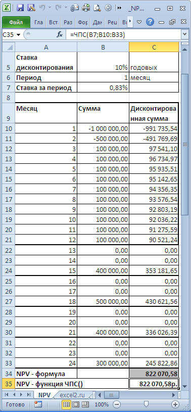
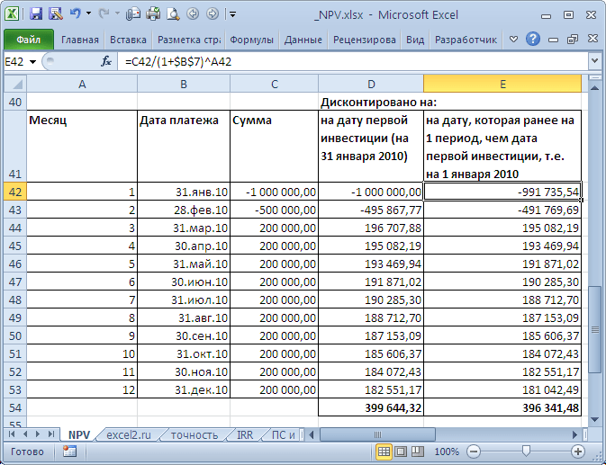
In the table, NPV is calculated in two ways: through the NPV() function and by formulas (calculating the present value of each amount). The table shows that already the first amount (investment) is discounted (-1,000,000 turned into -991,735.54). Let's assume that the first amount (-1,000,000) was transferred on January 31, 2010, which means its present value (-991,735.54=-1,000,000/(1+10%/12)) is calculated as of December 31, 2009. (without much loss of accuracy we can assume that as of 01/01/2010)
This means that all amounts are given not as of the date of transfer of the first amount, but at an earlier date - at the beginning of the first month (period). Thus, the formula assumes that the first and all subsequent amounts are paid at the end of the period.
If it is required that all amounts be given as of the date of the first investment, then it does not need to be included in the arguments of the NPV() function, but simply added to the resulting result (see example file).
A comparison of 2 discounting options is given in the example file, NPV sheet:
About the accuracy of calculating the discount rate
There are dozens of approaches for determining the discount rate. Many indicators are used for calculations: the weighted average cost of capital of the company; refinancing rate; average bank deposit rate; annual inflation rate; income tax rate; country risk-free rate; premium for project risks and many others, as well as their combinations. It is not surprising that in some cases the calculations can be quite labor-intensive. The choice of the right approach depends on the specific task; we will not consider them. Let us note only one thing: the accuracy of calculating the discount rate must correspond to the accuracy of determining the dates and amounts of cash flows. Let's show the existing dependency (see. example file, sheet Accuracy).
Let there be a project: implementation period is 10 years, discount rate is 12%, cash flow period is 1 year.
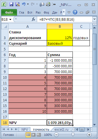
NPV amounted to 1,070,283.07 (Discounted to the date of the first payment).
Because If the project period is long, then everyone understands that the amounts in years 4-10 are not determined precisely, but with some acceptable accuracy, say +/- 100,000.0. Thus, we have 3 scenarios: Basic (the average (most “probable”) value is indicated), Pessimistic (minus 100,000.0 from the base) and Optimistic (plus 100,000.0 to the base). You must understand that if the base amount is 700,000.0, then the amounts of 800,000.0 and 600,000.0 are no less accurate.
Let's see how NPV reacts when the discount rate changes by +/- 2% (from 10% to 14%):

Consider a 2% rate increase. It is clear that as the discount rate increases, NPV decreases. If we compare the ranges of NPV spread at 12% and 14%, we see that they intersect at 71%.

Is it a lot or a little? Cash flow in years 4-6 is predicted with an accuracy of 14% (100,000/700,000), which is quite accurate. A change in the discount rate by 2% led to a decrease in NPV by 16% (when compared with the base case). Taking into account the fact that the NPV ranges overlap significantly due to the accuracy of determining the amounts of cash income, an increase of 2% in the rate did not have a significant impact on the NPV of the project (taking into account the accuracy of determining the amounts of cash flows). Of course, this cannot be a recommendation for all projects. These calculations are provided as an example.
Thus, using the above approach, the project manager must estimate the costs of additional calculations of a more accurate discount rate, and decide how much they will improve the NPV estimate.
We have a completely different situation for the same project, if the discount rate is known to us with less accuracy, say +/- 3%, and future flows are known with greater accuracy +/- 50,000.0
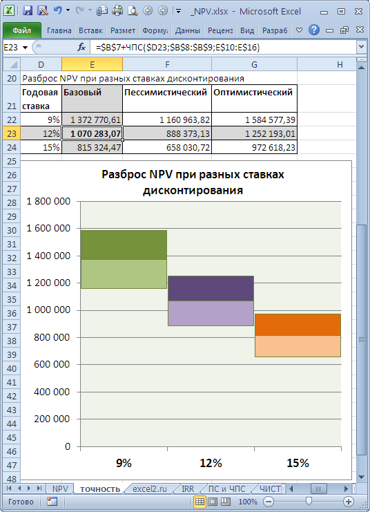
An increase in the discount rate by 3% led to a decrease in NPV by 24% (when compared with the base case). If we compare the ranges of NPV spread at 12% and 15%, we see that they intersect only by 23%.
Thus, the project manager, having analyzed the sensitivity of NPV to the discount rate, must understand whether the NPV calculation will be significantly refined after calculating the discount rate using a more accurate method.
After determining the amounts and timing of cash flows, the project manager can estimate what maximum discount rate the project can withstand (NPV criterion = 0). The next section talks about the Internal Rate of Return - IRR.
Internal rate of returnIRR(VSD)
Internal rate of return internal rate of return, IRR (IRR)) is the discount rate at which the Net Present Value (NPV) is equal to 0. The term Internal Rate of Return (IRR) is also used (see. example file, IRR sheet).
The advantage of IRR is that in addition to determining the level of return on investment, it is possible to compare projects of different scales and different durations.
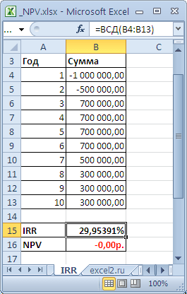
To calculate IRR, the IRR() function is used (English version - IRR()). This function is closely related to the NPV() function. For the same cash flows (B5:B14), the rate of return calculated by the IRR() function always results in a zero NPV. The relationship of functions is reflected in the following formula:
=NPV(VSD(B5:B14),B5:B14)
Note4. IRR can be calculated without the IRR() function: it is enough to have the NPV() function. To do this, you need to use a tool (the “Set in cell” field should refer to the formula with NPV(), set the “Value” field to 0, the “Changing cell value” field should contain a link to the cell with the rate).
Calculation of NPV with constant cash flows using the PS() function
Internal rate of return NET INDOH()
Similar to NPV(), which has a related function, IRR(), NETNZ() has a function, NETINDOH(), which calculates the annual discount rate at which NETNZ() returns 0.
Calculations in the NET INDOW() function are made using the formula:
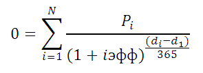
Where, Pi = i-th amount of cash flow; di = date of the i-th amount; d1 = date of 1st amount (starting date to which all amounts are discounted).
Note5. The function NETINDOH() is used for .
To assess the effectiveness of the project, the company's economists simulate the circulation of invested capital. In order to build models, cash flow and cash flow discounting methodologies are used. The basic parameter of the financial model of a project business plan is NPV, which we will consider in this article. This criterion came into economic analysis in the early nineties and to this day occupies the first position in the comprehensive and comparative assessment of projects.
Basics of project effectiveness assessment
Before we move directly to understanding NPV (net present value), I would like to briefly recall the main points of the evaluation methodology. Its key aspects make it possible to most competently calculate a group of project performance indicators, including NPV. Among the project participants, the main figure interested in evaluation activities is the investor. His economic interest is based on the awareness of the acceptable rate of return that he intends to extract from the actions of placing funds. The investor acts purposefully, refusing to consume available resources, and counts on:
- return of investment;
- compensation for your refusal in future periods;
- better conditions in comparison with possible investment alternatives.
By the rate of return beneficial to the investor, we will understand the minimum acceptable ratio of capital growth in the form of the company’s net profit and the amount of investment in its development. This ratio during the project period should, firstly, compensate for the depreciation of funds due to inflation, possible losses due to the occurrence of risk events, and secondly, provide a premium for abandoning current consumption. The size of this premium corresponds to the entrepreneurial interests of the investor.
The measure of entrepreneurial interest is profit. The best prototype of the profit generation mechanism for the purpose of evaluating an investment project is the flow methodology for reflecting cash flows (CF) from the perspective of income and expense parts. This methodology is called cash flow (CF or cash flow) in Western management practice. In it, income is replaced by the concepts of “receipts”, “inflows”, and expenses - “disposals”, “outflows”. The fundamental concepts of cash flow in relation to an investment project are: cash flow, settlement period and calculation step (interval).

Cash flow for investment purposes shows us the receipts of assets and their disposals arising in connection with project implementation during the entire duration of the billing period. The period of time during which it is necessary to track the cash flows generated by the project and its results in order to evaluate the effectiveness of the investment is called the calculation period. It represents a duration that may extend beyond the time frame of the investment project, including the transition and operational phases, until the end of the equipment life cycle. Planning intervals (steps) are usually calculated in years; in some cases, for small projects, a monthly interval breakdown can be used.
Methods for calculating net income
Of great importance for calculating NPV and other project indicators is how income and expenses are generated in the form of inflows and outflows of business assets. The cash flow methodology can be applied in a generalized form or localized by groups of cash flows (in operational, investment and financial aspects). It is the second form of representation that makes it possible to conveniently calculate net income as the simplest parameter for assessing efficiency. Next, we present to your attention a model of the relationship between the classical grouping of DS flows and grouping according to subject-target characteristics.

Scheme of two variants of groupings of DS flows with interconnections
The nature of the content of the economic effect of investments is expressed in the comparison of the total inflows and outflows of funds at each calculated step of the project task. Net income (CF or BH) is calculated for the corresponding interval value i. Below are the formulas for calculating this indicator. The dynamics of black holes are almost always repeated from project to project. For the first one or two steps, the ND value is negative, because the results of operating activities are not able to cover the size of the investments made. Then the sign changes, and in subsequent periods net income increases.

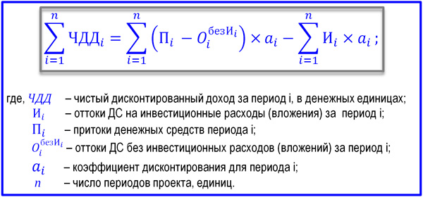
Formula for calculating net income for period i
The cost of DS changes over time. This is due not only to inflation, but also to the fact that money itself can generate a certain income. Therefore, the cash flow should be brought to the time of the start of the project through the discounting procedure, which uses the net present value method. Thanks to it, ND receives the status of a new indicator called “net present value” or “net present value”. We are no longer interested in step-by-step, but in cumulative discounted cash flow. Its formula is presented below.

Formula for total discounted cash flow
A separate material will be devoted to the parameters “discount rate”, “discounted cash flow”, “discount factor”, revealing their financial and economic nature. I will only note that guidelines for the value of r in a project can be the levels of the WACC indicator, the Central Bank refinancing rates, or the rate of return for an investor who is able to secure more profitable alternative investments. The total discounted cash flow can be interpreted and the net present value (NPV) can be calculated from it.
NPV formula
NPV shows us how much money an investor will be able to receive after the size of investments and regular outflows reduced to the initial moment are covered by the same inflows. The “net present value” indicator serves as a successful replica of the Western NPV indicator, which became widespread in Russia during the “boom” of business planning. In our country, this indicator is also called “net present value”. Both English and Russian interpretations of the NPV indicator are equally widespread. The NPV formula is shown below.
NPV formula for the purpose of assessing the effectiveness of a project activity
The net present value presented in the formula is the subject of much debate among practitioners. I do not pretend to have the truth, but I believe that domestic methodologists will have to bring some clarity to a number of issues and, perhaps, even correct textbooks. I will express only a couple of comments regarding the main nuances.
- To calculate the “net present value” indicator, one should rely on the classical understanding of net cash flow (NCF) as a combination of operating, investment and financial flows. But investments should be separated from NCF, since common sense discount factors may be different for the two parts of this formula.
- When calculating NPV (NPV), dividends associated with the project must be excluded from the NCF, since they serve as a form of withdrawal of the investor’s final income and should not affect the NPV value of the project.
Net present value, based on these comments, can have several interpretations of the formula, one of which is the option when the discount rate in relation to the size of the investment is based on the WACC or the percentage of inflation. At the same time, the base part of the NCF, reduced to the initial period at the rate of return, significantly reduces the net present value. The investor’s increased demands on the level of rate r has its consequences, and the net present value decreases or even reaches negative values.
Net present value is not an exclusive indicator of performance and should not be considered in isolation from a group of other criteria. However, NPV represents a major evaluation parameter due to its ability to express the economic impact of a project. Even if the indicator turns out to be slightly above zero, the project can already be considered effective. The formula for calculating NPV in the traditional form of the Western school of management is presented below.

Formula for the net present value of a project
Example of NPV calculation
As we have established, the discount factor carries the investor’s expectations for income from the project. And if during the billing period all project costs are covered by income taking into account discounting, the event is able to satisfy these expectations. The sooner such a moment comes, the better. The higher the net present value, the more effective the project. NPV shows how much additional income an investor can expect. Let's consider a specific example of NPV calculation. Its main initial conditions are:
- the value of the calculation period is 6 years;
- selected planning step – 1 year;
- the moment of starting investment corresponds to the beginning of step “0”;
- the need to obtain borrowed funds is ignored; for simplicity, we assume that investments were made at the expense of the company’s own capital, i.e. CF from financing activities is not taken into account;
- Two options for the discount rate are considered: option A, where r=0.1; option B, where r=0.2.
All initial data on investments and operating CF by project year are given in the table presented.
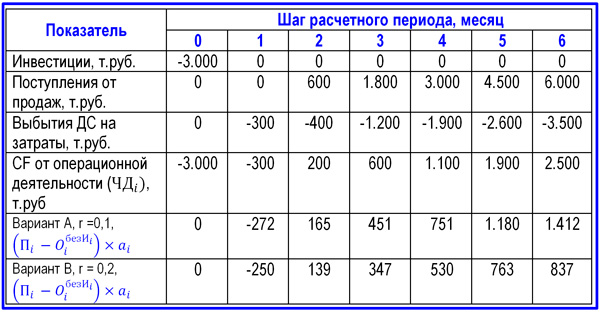
Example data for calculating the NPV of a project
As a result of filling out the bottom three rows of the table, we are able to calculate the indicators.
- The net income of the project amounted to 3,000 thousand rubles (-300+200+600+1100+1900+2500-3000).
- Net present value for r=0.1, amounting to 687 thousand rubles (-272+165+451+751+1180+1412-3000).
- For the discount rate, r=0.2 amounts to -634 thousand rubles (-250+139+347+530+763+837-3000).
If we compare the three obtained values, the conclusion suggests itself that with a rate of return of 10%, the project can be considered effective, while the investor’s demands for a rate of 20% exclude this event from the zone of his interests. This happens quite often. In recent years, in our economy, the value of the real rate of return has been steadily declining, so relatively few strategic investors come, mainly speculative ones.
In this article, we examined the most popular indicator of assessment, analysis of the economic efficiency of investments and project practice - NPV. When calculating the indicator, the net present value method is used, which allows you to adjust the cash flows generated in the project to changes in the time value of money. The advantage of this criterion is its ability to find an investment effect that is adequate to economic realities, and the disadvantage is its closeness to the investor’s subjective view of the level of expected profitability.
The Net present value, or NPV, indicator of an investment project allows you to determine what income the investor will receive in monetary terms as a result of his investments. In other words, the NPV of a project shows the amount of financial income as a result of investments in an investment project, taking into account associated costs, that is, net present value. What NPV is in practice and how to calculate net present value will become clear from the NPV formula below and its explanations.
Concept and content of NPV value
Before moving on to the topic of NPV, talking about what it is and how to calculate it, you need to understand the meaning of the phrase that makes up the abbreviation. For the phrase “Net present value” in the domestic economic and mathematical literature you can find several traditional translation options:
- In the first version, typical for mathematical textbooks, NPV is defined as net present value (NPV).
- The second option - net present value (NPV) - along with the first, is considered the most used.
- The third option – net present value – combines elements of the first and second transfers.
- The fourth version of the translation of the term NPV, where PV is “current value,” is the least common and is not widely used.
Regardless of the translation, the NPV value remains unchanged, and this term means that
NPV is the net present value of value. That is, cash flow discounting is precisely considered as the process of establishing its (flow) value by bringing the cost of total payments to a certain (current) point in time. Therefore, determining the value of net present value (NPV) becomes, along with IRR, another way to assess the effectiveness of investment projects in advance.
At the level of the general algorithm, in order to determine the prospects of a business project according to this indicator, the following steps need to be taken:
- assess cash flows – initial investments and expected receipts,
- set the cost of capital - calculate the rate,
- discount incoming and outgoing cash flows at an established rate,
- sum up all discounted flows, which will give the NPV value.
If the NPV calculation shows values greater than zero, then the investment is profitable. Moreover, the larger the NPV number, the greater, other things being equal, the expected profit value. Given that the lenders' return is usually fixed, anything the project brings in above it belongs to the shareholders - with a positive NPV, the shareholders will earn. The opposite situation with NPV less than zero promises losses for investors.
It is possible that the net present value will be zero. This means that the cash flow is sufficient to replace the invested capital without profit. If a project with an NPV of zero is approved, the size of the company will increase, but the share price will remain unchanged. But investing in such projects may be related to the social or environmental objectives of the initiators of the process, which makes investing in such projects possible.
NPV formula
Net present value is calculated using a calculation formula, which in a simplified form looks like PV - ICo, where PV represents the current cash flow indicators, and ICo is the size of the initial investment. In a more complex form, which shows the discounting mechanism, the formula looks like this:
NPV= - ICo + ∑ n t=1 CF t / (1 + R) t
 Here:
Here:
- NPV– net present value.
- CF – Cash Flow is the cash flow (investment payments), and t next to the indicator is the time during which the cash flow occurs (for example, an annual interval).
- R – Rate– discount (rate: coefficient that discounts flows).
- n– the number of stages of project implementation, which determines the duration of its life cycle (for example, the number of years).
- ICo – Invested Capital– initial invested capital.
Thus, NPV is calculated as the difference between the total cash flows updated at a certain point in time by risk factors and the initial investment, that is, investor profit is considered as the added value of the project.
Since it is important for an investor not only to make a profitable investment, but also to competently manage capital over a long period of time, this formula can be further expanded to include not one-time, but additional periodic investments and an inflation rate (i)
NPV= ∑ n t=1 CF t / (1 + R) t - ∑ m j =1 IC j / (1 + i) j
Example of NPV calculation
An example calculation for three conditional projects allows you to both calculate NPV and determine which of the projects will be more attractive for investment.
According to the example conditions:
- initial investments - ICo - in each of the three projects are equal to 400 USD,
- the rate of return - the discount rate - is 13%,
- the profits that projects can bring (by year) are listed in the table for a 5-year period.

Let's calculate net present value to choose the most profitable project for investment. The discount factor 1/(1 + R) t for an interval of one year will be t = 1: 1/(1+0.13)1 = 0.885. If we recalculate the NPV of each scenario by year with the substitution of the defining values into the formula, it turns out that for the first project NPV = 0.39, for the second – 10.41, for the third – 7.18.


According to this formula, the second project has the highest net present value, therefore, if we are based only on the NPV parameter, then it will be the most attractive for investment in terms of profit.
However, the projects being compared may have different durations (life cycles). Therefore, there are often situations when, for example, when comparing three-year and five-year projects, the NPV will be higher for the five-year one, and the average value over the years will be higher for the three-year one. To avoid any contradictions, the average annual rate of return (IRR) must also be calculated in such situations.
In addition, the volume of initial investment and expected profit are not always known, which creates difficulties in applying calculations.
Difficulties in applying calculations
As a rule, in reality, the variables read (substituted into the formula) are rarely accurate. The main difficulty is determining two parameters: the assessment of all cash flows associated with the project and the discount rate.
Cash flows are:
- initial investment – initial outflow of funds,
- annual inflows and outflows of funds expected in subsequent periods.
Taken together, the amount of flow indicates the amount of cash that an enterprise or company has at its disposal at the current moment in time. It is also an indicator of the financial stability of the company. To calculate its values, you need to subtract Cash Outflows (CO), the outflow, from the value of Cash Inflows (CI) - cash inflow:
 When forecasting potential revenues, it is necessary to determine the nature and degree of dependence between the influence of factors that form cash flows and the cash flow itself. The procedural complexity of a large complex project also lies in the amount of information that needs to be taken into account. So, in a project related to the release of a new product, it will be necessary to predict the volume of expected sales in units, while simultaneously determining the price of each unit sold. And in the long term, in order to take this into account, it may be necessary to base forecasts on the general state of the economy, the mobility of demand depending on the development potential of competitors, the effectiveness of advertising campaigns and a host of other factors.
In terms of operational processes, it is necessary to predict expenses (payments), which, in turn, will require an assessment of prices for raw materials, rental rates, utilities, salaries, exchange rate changes in the foreign exchange market and other factors. Moreover, if a multi-year project is planned, then estimates should be made for the corresponding number of years in advance.
If we are talking about a venture project that does not yet have statistical data on production, sales and costs, then forecasting cash income is carried out on the basis of an expert approach. It is expected that experts should compare a growing project with its industry counterparts and, together with the development potential, assess the possibilities of cash flows.
R – discount rate
The discount rate is a kind of alternative return that an investor could potentially earn. By determining the discount rate, the value of the company is assessed, which is one of the most common purposes for establishing this parameter.
The assessment is made based on a number of methods, each of which has its own advantages and initial data used in the calculation:
- CAPM model. The technique allows you to take into account the impact of market risks on the discount rate. The assessment is made on the basis of trading on the MICEX exchange, which determines the quotations of ordinary shares. In its advantages and choice of initial data, the method is similar to the Fama and French model.
- WACC model. The advantage of the model is the ability to take into account the degree of efficiency of both equity and borrowed capital. In addition to the quotations of ordinary shares, interest rates on borrowed capital are taken into account.
- Ross model. Makes it possible to take into account macro- and microfactors of the market, industry characteristics that determine the discount rate. Rosstat statistics on macroindicators are used as initial data.
- Methods based on return on equity, which are based on balance sheet data.
- Gordon model. Using it, an investor can calculate dividend yield, also based on quotes of ordinary shares, and also other models.
Changes in the discount rate and the amount of net present value are related to each other by a nonlinear relationship, which can simply be reflected on a graph. This implies a rule for the investor: when choosing a project - an investment object - you need to compare not only the NPV values, but also the nature of their change depending on the rate values. The variability of scenarios allows an investor to choose a less risky project for investment.

Since 2012, at the instigation of UNIDO, the calculation of NPV has been included as an element in the calculation of the index of the rate of specific increase in value, which is considered the optimal approach when choosing the best investment decision. The assessment method was proposed by a group of economists headed by A.B. Kogan, in 2009. It allows you to effectively compare alternatives in situations where it is not possible to compare using a single criterion, and therefore the comparison is based on different parameters. Such situations arise when the analysis of investment attractiveness using traditional NPV and IRR methods does not lead to unambiguous results or when the results of the methods contradict each other.
Net Present Value (NPV) Method- one of the most commonly used methods for estimating cash flows.
Among the others - methods of cash flow for share capital and cash flow for total invested capital.
When calculating the weighted average cost of capital, each type of capital, whether ordinary or preferred shares, bonds or long-term debt, is taken into account with its corresponding weights. An increase in the weighted average cost of capital usually reflects an increase in risks.
To avoid double counting of these tax shields, interest payments should not be deducted from cash flows.
Equation 4.1 shows how to calculate cash flows (subscripts correspond to time periods):
- CF CF t = EBIT t * (1 - τ) + DEPR t - CAPEX t - ΔNWC t + other t, (4.1)
- - cash flows; EBIT
- τ - earnings before interest and taxes;
- - income tax rate; DEPR
- - depreciation; CAPEX
- - capital expenditures;- increase in net working capital;
- other- increase in tax arrears, wage arrears, etc.
Then you need to calculate the terminal value. This valuation is very important because much of the value of a company, especially a start-up, can be contained in the terminal value. The generally accepted method of calculating the terminal value of a company is the perpetual growth method.
Equation 4.2 provides the formula for terminal value (TV) calculation at time τ using the perpetual growth method with perpetual growth rates g and discount rate r.
Cash flows and discount rates used in the NPV method are usually represented by nominal values ( that is, they are not adjusted for inflation).
If cash flow is projected to be constant in inflation-adjusted dollar terms, a post-forecast growth rate equal to the inflation rate should be used:
TV T = / (r - g). (4.2)
Other commonly used methods for calculating terminal value in practice use price-earnings ratios and market-to-book ratios, but such simplifications are discouraged. The company's net present value is then calculated according to the formula in Equation 4.3:
NPV= + + +
+... + [(CF T + TV T) / (l + r) T ]. (4.3)
The discount rate is calculated using equation 4.4:
r = (D / V) * r d * (1 - τ) + (E / V) * r e, (4.4)
- r d- discount rate for debt;
- r e
- τ - earnings before interest and taxes;
- D- market value of debt;
- E
- V- D + E.
Even if a company's capital composition does not meet the target capital composition, target values for D/V and E/V must be used.
The cost of equity (g) is calculated using the financial asset pricing model (CAPM), see equation 4.5:
r e = r f + β * (r m - r f), (4.5)
- r e- discount rate for share capital;
- r f- risk-free rate;
- β - beta or degree of correlation with the market;
- r m- market rate of return on ordinary shares;
- (r m - r f)- risk premium.
When determining a reasonable risk-free rate (rf), it is necessary to try to correlate the degree of maturity of the investment project with the risk-free rate. Typically a ten-year rate is used. Estimates of the risk premium can vary greatly: for ease of understanding, you can take the value of 7.5%.
For non-public companies or companies spun off from public companies, beta can be approximated by taking public company peers as an example. Beta for public companies can be found in the Beta Book or Bloomberg.
If a company has not achieved its target capital composition, it is necessary to unleverage beta and then calculate beta taking into account the company's target debt-to-equity ratio. How to do this is shown in Equation 4.6:
β u = β l * (E / V) = β l * , (4.6)
- β u- beta coefficient without financial leverage;
- β l- beta coefficient taking into account financial leverage;
- E- market value of share capital;
- D- market value of debt.
The problem arises if there are no comparable companies, which often happens in situations with non-public companies. In this case, it is best to use common sense. You need to think about the cyclical nature of a particular company and whether the risk is systematic or can be diversified away.
If financial statement data is available, an "earnings beta" can be calculated, which has some correlation with equity beta. Earnings beta is calculated by comparing a non-public company's net earnings to a stock index such as the S&P 500.
Using the least squares regression technique, you can calculate the slope of the line of best fit (beta).
A sample net present value calculation is provided below.
Example of valuation using the net present value method
Lo-Tech shareholders voted to stop diversification and decided to refocus on core business areas. As part of this process, the company would like to sell Hi-Tech, its startup high-tech subsidiary.
Hi-Tech executives, who wanted to acquire the company, turned to George, a venture capitalist, for advice. He decided to value Hi-Tech using the net present value method. George and Hi-Tech management agreed on the forecasts presented in the table (all data are in millions of dollars).
Input data for analysis using the net present value method (millions/dollars)
The company has net operating losses of $100 million that can be carried forward and offset by future earnings. Additionally, Hi-Tech is projected to generate further losses in its early years of operations.
She will also be able to carry these losses forward to future periods. The tax rate is 40%.
The average non-leveraged beta of the five technology peers is 1.2. Hi-Tech has no long-term debt. The 10-year US Treasury yield is 6%.
It is assumed that the required capital expenditure will be equal to the amount of depreciation. The risk premium assumption is 7.5%. Net working capital is projected to be 10% of sales. EBIT is projected to grow 3% per year in perpetuity beyond Year 9.
As shown in the table below, George first calculated the weighted average cost of capital:
WACC = (D / V) * r d * (1 - t) + (E / V) * r e =
= 0 + 100% * = 15%.
Net Present Value Analysis
(millions of dollars)
Calculation of the weighted average cost of capital
|
Less: costs |
||||||||||
|
Less: tax |
||||||||||
|
EBIAT (earnings before interest and after taxes) |
||||||||||
|
Less: change. net working capital |
||||||||||
|
Free Cash Flow |
-104 | |||||||||
|
Coefficient discounting |
||||||||||
|
Present value (cash flow) |
||||||||||
|
Terminal cost |
||||||||||
Net present value and sensitivity analysis.
Weighted average cost of capital (WACC)
|
Present value (cash flows) |
|||||||||
|
Present value (terminal value) |
Growth rates in the post-forecast period |
||||||||
|
Net present value |
|||||||||
|
Tax calculation |
|||||||||
|
Pure operas used. losses |
|||||||||
|
Added pure operas. losses |
|||||||||
|
Pure operas. losses at the beginning of the period |
|||||||||
|
Pure operas. losses at the end of the period |
|||||||||
|
Net working capital (10% of sales) |
|||||||||
|
Net working capital at the beginning of the period |
|||||||||
|
Net working capital at the end of the period |
|||||||||
|
Change net circulating capital |
|||||||||
He then estimated the cash flows and found the company's net present value to be $525 million. As expected, the entire value of the company was contained in the terminal value ( the present value of the cash flows was -$44 million, and given the NPV of the terminal value of $569 million, the NPV was $525 million).
The terminal value was calculated as follows:
TV T = / (r - g) =
= / (15% - 3%) - $2,000.
George also performed a scenario analysis to determine the sensitivity of Hi-Tech's valuation to changes in the discount rate and growth rate in the post-forecast period. He compiled a table of scenarios, which is also presented in the table.
George's scenario analysis produced a series of values ranging from $323 million to $876 million. Of course, such a wide spread could not be an accurate guide to the real value of Hi-Tech.
He noted that negative initial cash flows and positive future cash flows made the valuation very sensitive to both changes in the discount rate and changes in growth rates in the post-forecast period.
George viewed the net present value method as the first step in the valuation process and planned to use other methods to narrow the range of possible values for Hi-Tech.
Advantages and disadvantages of the net present value method
Estimating the value of a company by discounting the relevant cash flows is considered a technically sound method. Compared to the analogue method, the resulting estimates should be less susceptible to distortions that occur in the market for public and, even more often, non-public companies.
Given the numerous assumptions and calculations that are made during the estimation process, however, it is unrealistic to arrive at a single or “point” value. Various cash flows must be assessed using the best case, best case and worst case scenarios.
They should then be discounted using a range of values for the weighted average cost of capital and the post-forecast growth rate (g) to arrive at a likely range of estimates.
If you can set the probability of occurrence for each scenario, the weighted average will correspond to the expected value of the company.
But even with such adjustments, the net present value method is not without some drawbacks. First of all, to calculate the discount rate, we need beta coefficients.
A suitable peer company should demonstrate similar financial performance, growth prospects and operating characteristics as the company we are evaluating. A public company with these characteristics may not exist.
Target capital composition is often also estimated using peers, and using peer companies to estimate target capital composition has many of the same disadvantages as looking for similar betas. Additionally, the typical cash flow profile of a startup—large expenses early on and revenues far into the future—means that most (if not all of the value) is in terminal value.
Terminal value values are very sensitive to assumptions about discount rates and growth rates in the post-forecast period. Finally, recent research in the financial industry has raised questions about the validity of beta as a valid measure of a company's risk.
Numerous studies have suggested that company size or the market-to-book ratio might be more appropriate values, but in practice few have attempted to apply such an approach to company valuation.
Another disadvantage of the net present value method becomes apparent when valuing companies with changing capital composition or effective tax rates.
Changing capital composition is often associated with highly leveraged transactions, such as leveraged buyouts.
Effective tax rates may change due to the use of tax deductions, such as for net operating losses, or the cessation of tax subsidies that are sometimes available to young and fast-growing companies.
When using the net present value method, capital composition and the effective tax rate are taken into account in the discount rate (WACC), while assuming that they are constant values. Due to the reasons listed above, it is recommended to use the adjusted present value method in these cases.
NPV is an abbreviation for the first letters of the phrase “Net Present Value” and stands for net present value (to date). This is a method of evaluating investment projects based on the discounted cash flow methodology. If you want to invest money in a promising business project, then it would be a good idea to first calculate the NPV of this project. The calculation algorithm is as follows:
- you need to estimate the cash flows from the project - the initial investment (outflow) of funds and the expected receipts (inflows) of funds in the future;
- determine the cost of capital Cost of Capital) for you - this will be the discount rate;
- discount all cash flows (inflows and outflows) from the project at the rate that you estimated in step 2);
- Fold. The sum of all discounted flows will be equal to the NPV of the project.
If NPV is greater than zero, then the project can be accepted; if NPV is less than zero, then the project should be rejected.
The rationale behind the NPV method is very simple. If the NPV is zero, this means that the cash flows from the project are sufficient to:
- recoup invested capital and
- provide the necessary income on this capital.
If the NPV is positive, it means that the project will bring profit, and the higher the NPV value, the more profitable the project is for the investor. Since the income of the creditors (who you borrowed money from) is fixed, all income above this level belongs to the shareholders. If the company approves a project with zero NPV, the shareholders' position will remain unchanged - the company will become larger, but the share price will not increase. However, if the project has a positive NPV, the shareholders will become richer.
NPV calculation. Example
The formula for calculating NPV looks complicated to a person who does not consider himself a mathematician: 
Where
- n, t — number of time periods;
- CF - cash flow Cash Flow);
- R is the cost of capital, also known as the discount rate. Rate).
In fact, this formula is just a correct mathematical representation of the summation of several quantities. To calculate NPV, let's take two projects as an example A And B, which have the following cash flow structure for the next 4 years:
Table 1. Cash flow of projects A and B.
| Year | Project A | Project B |
|---|---|---|
| 0 | ($10,000) | ($10,000) |
| 1 | $5,000 | $1,000 |
| 2 | $4,000 | $3,000 |
| 3 | $3,000 | $4,000 |
| 4 | $1,000 | $6,000 |
Both projects A And B have the same initial investment of $10,000, but the cash flows in subsequent years are very different. Project A assumes a faster return on investment, but by the fourth year the cash flow from the project will drop significantly. Project B, on the contrary, in the first two years shows lower cash inflows than the proceeds from the Project A, but in the next two years the Project B will bring more money than the project A. Let's calculate the NPV of the investment project.
To simplify the calculation, let's assume:
- all cash flows occur at the end of each year;
- the initial cash outflow (investment of money) occurred at time “zero”, i.e. Now;
- The cost of capital (discount rate) is 10%.
Let us recall that in order to bring the cash flow to today, you need to multiply the amount of money by the coefficient 1/(1+R), while (1+R) must be raised to a power equal to the number of years. The value of this fraction is called the factor or discount factor. In order not to calculate this factor every time, you can look it up in a special table called the “discount factor table.”
Let's apply the NPV formula for the Project A. We have four annual periods and five cash flows. The first flow ($10,000) is our investment at time zero, that is, today. If we expand the NPV formula given just above, we get a sum of five terms:
If we substitute the data from the table for the Project into this amount A instead of CF and a rate of 10% instead R, then we get the following expression:
What is in the divisor can be calculated, but it is easier to take the ready-made value from the table of discount factors and multiply these factors by the amount of cash flow. As a result, the present value of cash flows for the project A equal to $788.2. NPV calculation for a project A can also be presented in table form and as a time scale:
| Year | Project A | Rate 10% | Factor | Sum |
|---|---|---|---|---|
| 0 | ($10,000) | 1 | 1 | ($10,000) |
| 1 | $5,000 | 1 / (1.10) 1 | 0.9091 | $4,545.5 |
| 2 | $4,000 | 1 / (1.10) 2 | 0.8264 | $3,305.8 |
| 3 | $3,000 | 1 / (1.10) 3 | 0.7513 | $2,253.9 |
| 4 | $1,000 | 1 / (1.10) 4 | 0.6830 | $683.0 |
| TOTAL: | $3,000 | $788.2 |

Figure 1. NPV calculation for project A.
Let's calculate NPV for the project in a similar way B.
Because discount factors decrease over time, the contribution to the present value of the project from large ($4,000 and $6,000) but distant (years 3 and 4) cash flows will be less than the contribution from cash flows in the early years of the project. Therefore, it is expected that for the project B the net present value of the cash flows will be less than for the project A. Our NPV calculations for the project B gave the result - $491.5. Detailed NPV calculation for the project B shown below.
Table 2. NPV calculation for project A.
| Year | Project B | Rate 10% | Factor | Sum |
|---|---|---|---|---|
| 0 | ($10,000) | 1 | 1 | ($10,000) |
| 1 | $1,000 | 1 / (1.10) 1 | 0.9091 | $909.1 |
| 2 | $3,000 | 1 / (1.10) 2 | 0.8264 | $2,479.2 |
| 3 | $4,000 | 1 / (1.10) 3 | 0.7513 | $3,005.2 |
| 4 | $6,000 | 1 / (1.10) 4 | 0.6830 | $4,098.0 |
| TOTAL: | $4,000 | $491.5 |

Figure 2. NPV calculation for project B.
Conclusion
Both of these projects can be accepted, since the NPV of both projects is greater than zero, which means the implementation of these projects will lead to an increase in the income of the investor company. If these projects are mutually exclusive and you need to choose only one of them, then the project looks preferable A, since its NPV=$788.2, which is greater than the NPV=$491.5 of the project B.
Subtleties of NPV calculation
Applying a mathematical formula is not difficult if all the variables are known. Once you have all the numbers - cash flows and cost of capital, you can easily plug them into the formula and calculate NPV. But in practice it is not so simple. Real life differs from pure mathematics in that it is impossible to accurately determine the magnitude of the variables that enter into this formula. As a matter of fact, this is why in practice there are many more examples of unsuccessful investment decisions than successful ones.
Cash flows
The most important and most difficult step in analyzing investment projects is assessing all the cash flows associated with the project. Firstly, this is the amount of the initial investment (outflow of funds) today. Secondly, these are the amounts of annual cash inflows and outflows that are expected in subsequent periods.
Making an accurate forecast of all the costs and revenues associated with a large, complex project is incredibly difficult. For example, if an investment project is associated with the launch of a new product on the market, then to calculate NPV it will be necessary to make a forecast of future sales of the product in units and estimate the sales price per unit of product. These forecasts are based on an assessment of the general state of the economy, the elasticity of demand (the dependence of the level of demand on the price of a product), the potential effect of advertising, consumer preferences, and the reaction of competitors to the launch of a new product.
In addition, it will be necessary to make a forecast of operating expenses (payments), and for this to estimate future prices for raw materials, employee salaries, utilities, changes in rental rates, trends in changes in exchange rates, if some raw materials can only be purchased abroad, etc. Further. And all these assessments need to be made several years in advance.
Discount rate
The discount rate in the NPV calculation formula is the cost of capital for the investor. In other words, this is the interest rate at which the investing company can attract financial resources. In general, a company can obtain financing from three sources:
- borrow (usually from a bank);
- sell your shares;
- use internal resources (for example, retained earnings).
The financial resources that can be obtained from these three sources have their own costs. And she is different! The most clear is the cost of debt obligations. This is either the interest on long-term loans that banks require, or the interest on long-term bonds if the company can issue its debt instruments in the financial market. It is more difficult to estimate the cost of financing from the other two sources. Financiers have long developed several models for such an assessment, among them the well-known CAPM(Capital Asset Pricing Model). But there are other approaches.
The company's cost of capital (and therefore the discount rate in the NPV formula) will be the weighted average of the interest rates from these three sources. In English financial literature this is referred to as WACC(Weighted Average Cost of Capital), which translates as the weighted average cost of capital.
Dependence of the NPV of the project on the discount rate
It is clear that obtaining absolutely accurate values of all cash flows of the project and accurately determining the cost of capital, i.e. discount rate is not possible. In this regard, it is interesting to analyze the dependence of NPV on these values. It will be different for each project. The most frequently performed analysis is the sensitivity of the NPV indicator to the cost of capital. Let's calculate NPV for projects A And B for different discount rates:
| Cost of capital, % | NPV A | NPV B |
|---|---|---|
| 0 | $3,000 | $4,000 |
| 2 | $2,497.4 | $3,176.3 |
| 4 | $2,027.7 | $2,420.0 |
| 6 | $1,587.9 | $1,724.4 |
| 8 | $1,175.5 | $1,083.5 |
| 10 | $788.2 | $491.5 |
| 12 | $423.9 | ($55.3) |
| 14 | $80.8 | ($562.0) |
| 16 | ($242.7) | ($1,032.1) |
| 18 | ($548.3) | ($1,468.7) |
Table 3. Dependence of NPV on the discount rate.
The tabular form is inferior to the graphical form in terms of information content, so it is much more interesting to look at the results on the graph (click to enlarge the image):

Figure 3. Dependence of NPV on the discount rate.
The graph shows that the NPV of the project A exceeds the NPV of the project B at a discount rate of more than 7% (more precisely 7.2%). This means that an error in estimating the cost of capital for the investing company could lead to an erroneous decision regarding which of the two projects to choose.
In addition, the graph also shows that Project B is more sensitive to the discount rate. That is, the NPV of the project B decreases faster as this rate increases. And this is easy to explain. In project B Cash receipts in the first years of the project are small, but they increase over time. But discount rates for longer periods of time decrease very significantly. Therefore, the contribution of large cash flows to the net present value also drops sharply.
For example, you can calculate what $10,000 will be equal to in 1 year, 4 years and 10 years at discount rates of 5% and 10%, you can clearly see how much the present value of a cash flow depends on the time of its occurrence.
Table 4. Dependence of NPV on the time of its occurrence.
| Year | Rate 5% | Rate 10% | Difference, $ | Difference, % |
|---|---|---|---|---|
| 1 | $9,524 | $9,091 | $433 | 4.5% |
| 4 | $8,227 | $6,830 | $1,397 | 17.0% |
| 10 | $6,139 | $3,855 | $2,284 | 37.2% |
The last column of the table shows that the same cash flow ($10,000) at different discount rates differs after a year by only 4.5%. Whereas the same cash flow, only 10 years from today at a discount rate of 10%, will be 37.2% less than its present value at a discount rate of 5%. The high cost of capital “eats up” a significant part of the income from an investment project in distant annual periods, and nothing can be done about it.
That is why, when evaluating investment projects, cash flows that are more than 10 years distant from today are usually not used. In addition to the significant impact of discounting, the accuracy of estimating long-term cash flows is significantly lower.
Views: 14,942
Read also...
- Pin interpretation of the dream book Why do you dream of pins in your mouth
- Tasks for children to find an extra object
- Population of the USSR by year: population censuses and demographic processes All-Union Population Census 1939
- Speech material for automating the sound P in sound combinations -DR-, -TR- in syllables, words, sentences and verses